


This tutorial explains the basics of SUMIF and SUMIFS functions in LibreOffice Calc.
Table of Contents
SUMIF
SUMIF Function returns the sum total of the values from a range/list of cells based on a condition. For example, if you have a list of numbers in Calc and want to sum only the values which are less than 20, then you can use the SUMIF function.
Here are some examples that will help you understand the workings of SUMIF.
SUMIF Examples
Using Numbers
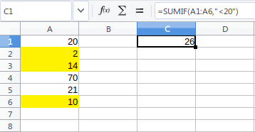
The below example sums the values from cells A1 to A6 if it is less than 20. The yellow highlighted values are the cells which are matching with the conditions.
=SUMIF(A1:A6,"<20”)
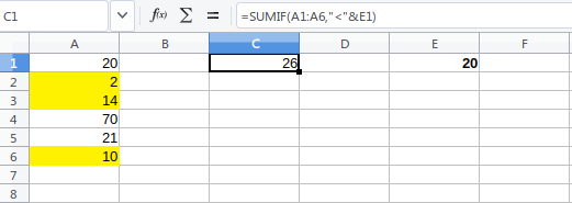
You can also keep the criteria value, i.e. 20 in a cell and use the cell reference in the SUMIF formula as below. It gives the same result as above.
=SUMIF(A1:A6,"<"&E1)
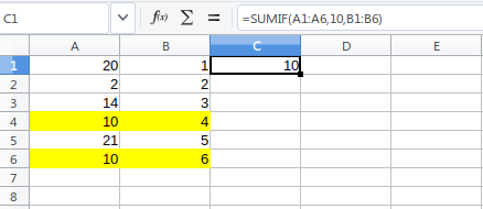
SUMIF can take three arguments where, based on the criteria, match in a range, you can sum another range. In the example below, it searches 10 in A1 to A6 and returns corresponding sums from range B1 to B6 if a match is found.
=SUMIF(A1:A6,10,B1:B6)
Similarly, you can put a value of 10 in any cell and use the cell reference in the above formula.
Using Texts
You can also search texts in a similar way and return the sum.
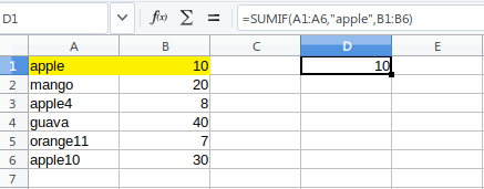
The following example searches “apple” in the range A1:A6 and returns the sum of matching entries from the corresponding sum range.
=SUMIF(A1:A6,"apple",B1:B6)
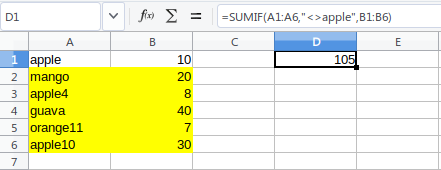
Using the condition below, you can sum the values that are NOT equal to a specific text/string. The NOT operator is <>. Please note that <> operator is inside the text with ".
=SUMIF(A1:A6,"<>apple",B1:B6)
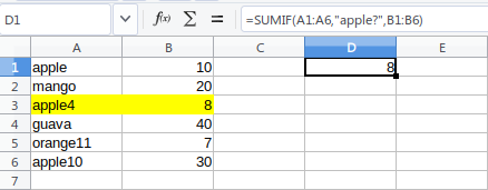
To search using a single wild card character, you can use ? in the condition. E.g. if you want to sum only strings matching with “apple4” and not “apple10” or “apple”, use the below example.
=SUMIF(A1:A6,"apple?",B1:B6)
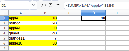
You can also use wild card * to search any number of characters in a range of cells and return the sum using SUMIF. The below example sums all matching cells where the apple word is found.
=SUMIF(A1:A6,"*apple*",B1:B6)
SUMIFS Example
You can use SUMIFS for multiple criteria ranges for summing up values. SUMIFS takes the first argument as the range to be summed and the next set of criteria as per the above examples.
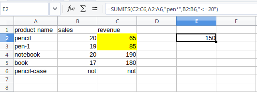
In the below example, it returns the sum of revenue when sales are less than or equal to 20, and the product name starts with pen.
=SUMIFS(C2:C6,A2:A6,"pen*",B2:B6,"<=20")
Note:
- SUMIFS conditions are evaluated as AND, and the sum is returned only when all conditions are satisfied.
- SUMIFS conditions ranges should be of the same length.
- You can specify at most 127 condition pairs in SUMIFS.
Summary
In conclusion, I guess this guide helped you to understand the working principles of SUMIF and SUMIFS. You can experiment with more conditions as per your need in LibreOffice Calc.
Drop a comment below if you have any questions or if this tutorial helped you.