This article explains two essential functions of REPLACE and SUBSTITUTE in LibreOffice Calc.
Often, you need to use the SUBSTITUTE function to replace a portion of a text in a cell. It can be in a single cell or a range of cells. So, to do that, you need to know these two functions. And with these two, you can easily manipulate any strings and get the desired result in no time.
Let’s find out.
Table of Contents
Replace and Substitute in LibreOffice Calc
SUBSTITUTE
Syntax
SUBSTITUTE (text, search text, new text, occurrence)
- Text: the target text where the search occurs
- Search text: The text to search
- New Text: The text to replace if the search is successful
- Occurrence: The occurrence of the matched text to replace (optional)
Example
I have a text that says, “LibreOffice is awesome”. Now I want to replace “awesome” with “great”. So, to do that, use this formula.
=SUBSTITUTE(B4,"great","awesome")

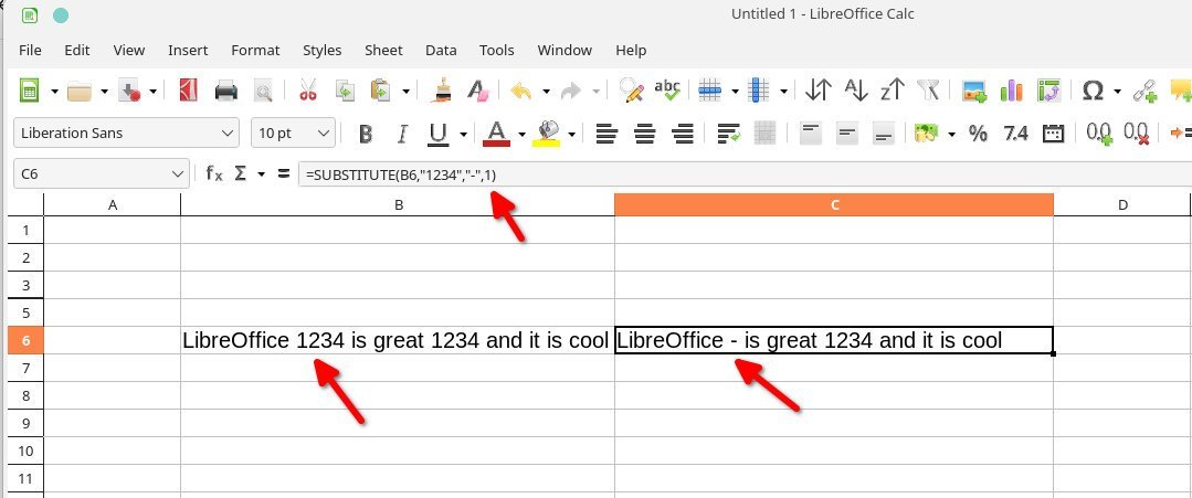
Let’s try with another example. Say we have the text “LibreOffice 1234 is great 1234, and it is cool”. What if we want to replace the “1234” occurrences with a character “-“.
So, to replace the 1st occurrence, you use the same formula but with the last parameter as 1 i.e. the occurrence of the first “1234”. This is how it works.
=SUBSTITUTE(B6,"1234","-",1)
If you want to replace the second occurrence, choose option 2 as a final parameter. But remember, it would not replace the first one.
Using this method, you can easily remove the texts if you use an empty string (“”) as a replacement character. In fact, you can remove spaces if you can find space and replace it with an empty string.
REPLACE
Syntax
REPLACE (text, position, length, new text)
- Text: the target text where the search occurs
- Position: Starting position of the search
- Length: The length of the text to replace
- New text: The text to replace a specified length
Example
To demonstrate, we prepared a set of random data with a numeric part and alphabets. So, what if we want to replace all the alphabets with empty strings to get a clean set of numeric data.
To do that, we used the below formula.
=REPLACE(B3,4,2,"")
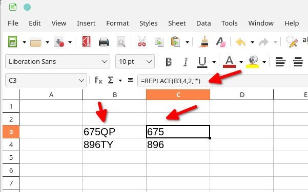
As you can see, the function searched from the 4th position and replaced the following two characters with empty spaces, leaving you just the numbers.
One of the crucial aspects to remember is that to change a column of data, you need to analyse whether the replacement part starts with the same position for the entire data set. So, be cautious while using this in that context.
Tip
IF you need byte-level manipulation, use the REPLACEB function. It works with the byte position instead of the character position.
Summary
I hope it helps you play around and clean up your data as per your need. Drop a note down below if you need help, or it helps you.
Official reference