Here are some of the ways you can find substring in LibreOffice Calc cells.
Table of Contents
How to Find Substring in LibreOffice Calc cell
First and foremost, no substring function is present in the LibreOffice Calc cell.
That means, you have to use the following functions (or combinations of them) while doing your work.
MID, LEFT, RIGHT, FIND, LEN, SUBSTITUTE, REPT, TRIM
In this article, I will explain some examples using the above functions. That would help you to understand you can find substring in LibreOffice Calc cell values.
Using MID Function
In the following example, there are three sentences. Each has a number enclosed by parenthesis. How can you extract the number only and put it on another cell?
I will use the MID function in this example. Here’s its syntax.
MID(search_text, start_number, length)

search_text: the cell value where you want to search. This can be a value or cell reference
start_number: from which number of character, substring will be returned. This must be a whole number.
length: the size of the substring to be returned. This must be a whole number.
To do that, I have used the below formula.
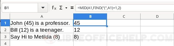
=MID(A1,FIND("(",A1)+1,2)
Explanation: Search will happen on the value of A1, and then I will find out the position of “(” – first parenthesis. That would be the starting position+1 of the substring. And the length to be returned is 2.
Here’s the result in this image.
But, there’s a problem in the 3rd row which returned the closing parenthesis. Because we have supplied the length as two and there is only one number.
How to fix this? Let’s modify the formula as below.
=MID(A1,FIND("(",A1)+1,FIND(")",A1)-FIND("(",A1)-1)
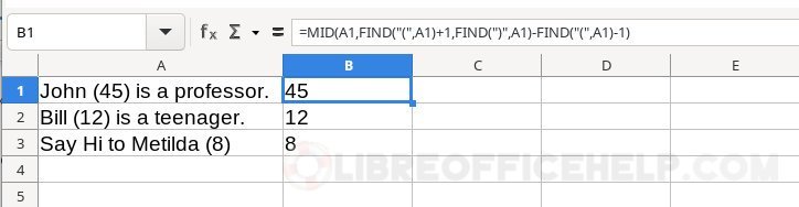
Explanation: The first two part of the formula is correct. The length formula is different here. I am finding the position of closing parenthesis “)” and then subtracting it from the position of “(“, by reducing one number. This eventually gives us the desired result.
Let’s see a complex example.
Using SUBSTITUTE and MID together
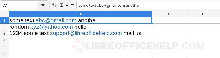
Here’s a sample of the data I have. It contains a mix of words with email addresses between them. How can you extract the email address only? Note that the length of the texts and email addresses are different. Hence you can not use the text to columns.
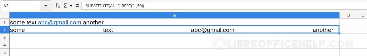
As a first step, I will separate the email address portion by adding many spaces, such as 50 spaces. To do that, I will use the SUBSTITUTE function to replace one single space ” ” with 50 spaces by using the REPT function.
=SUBSTITUTE(A1," ", REPT(" ",50))
And here’s the result if I apply this to the first cell data, i.e. A1. As you can see, the email address is now separated from the words. Each single space is replaced by 50 spaces.
The next step would be to remove all the words and keep only the email address with spaces. Since I have added 50 spaces (I know already that there are 50 spaces before and after the email addresses), it’s time to find the “@” using the MID function explained above.
The trick here is to approximate the spaces, excluding the words.
=MID(A2,FIND("@",A2)-25,75)

As you can see, the email address is separated from the words. But it had spaces. All you need to do is use the TRIM function to remove the spaces.
=TRIM(A3)

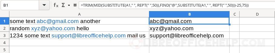
By combining all the steps, the final formula becomes this.
=TRIM(MID(SUBSTITUTE(A1," ", REPT(" ",50)),FIND("@",SUBSTITUTE(A1," ", REPT(" ",50)))-25,75))
And here’s the final result. It might look complex, but it is not – if you think about it.
Download the sample example spreadsheet here.
Wrapping Up
I have shown you how to find substring in LibreOffice Calc cells with various methods. It includes MID, LEFT, RIGHT and other functions. I hope this helps you understand its basics, which you can apply to your use case.
Do let me know in the comment box if you have any questions.