Lookup and Reference Functions in LibreOffice Calc

A simple beginner’s guide to lookup and reference functions in LibreOffice Calc.

LibreOffice Calc provides all the necessary lookup and reference functions for your day-to-day workflow and solving complex spreadsheet problems.

This article is a summary of all the necessary functions.

Table of contents

• VLOOKUP
• HLOOKUP
• MATCH and INDEX

Lookup and Reference in LibreOffice Calc

The lookup concept basically is to retrieve or find some values based on the “key” or reference. For example, if you have two sets of data with a common column, say “ID” of fruits as below. One table has the name and per kilo price. And another table has a subset of the fruits.

How can you get the names and calculate the total price by fetching relevant data from the other table?

VLOOKUP

VLOOKUP is an abbreviation of vertical lookup. So, to find out the names and other items in the above example, I will add the below formula to cell B2 using VLOOKUP. Here’s its syntax and formula.

Syntax of VLOOKUP

=VLOOKUP(search item, table array, column number of table array to be returned, search type)

search type: 0=Exact match; 1=Approximate match

Example formula

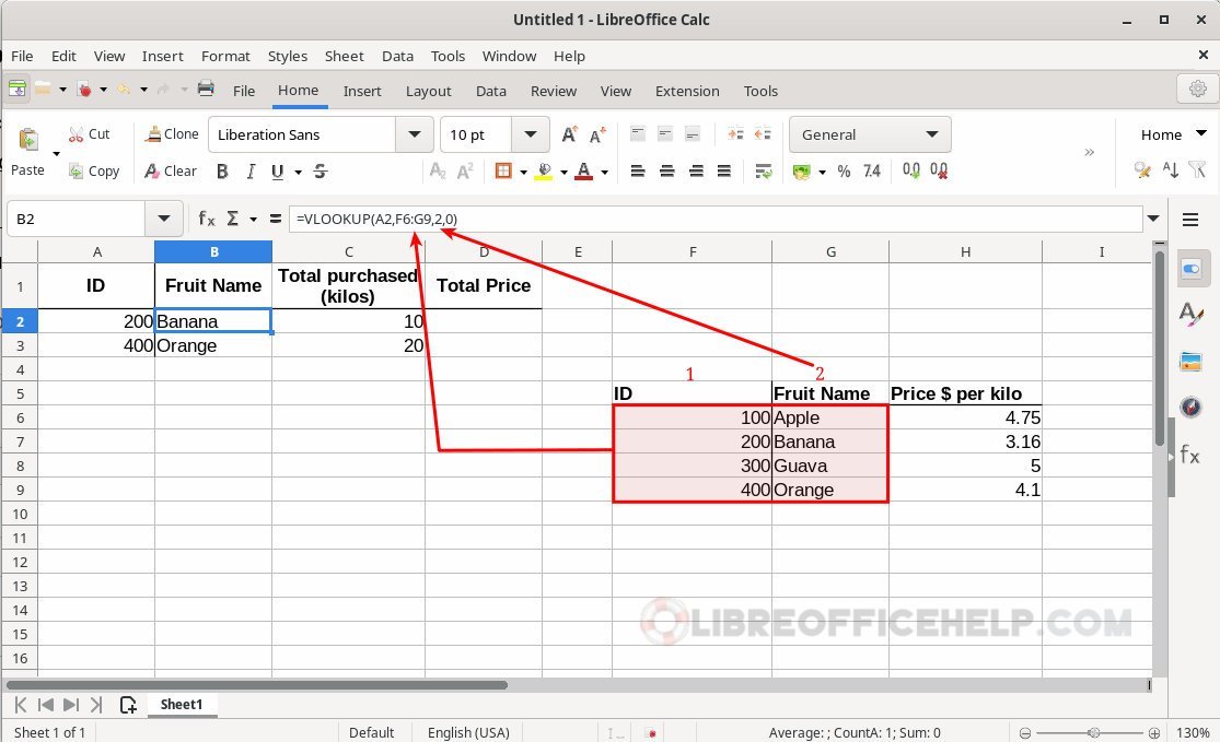
=VLOOKUP(A2,F6:G9,2,0)

Explanation: The formula search for ID at A2, i.e. "200" in table F6:G9, and returns the second column (“2”) of the selected table. Here’s a mockup of the explanation.

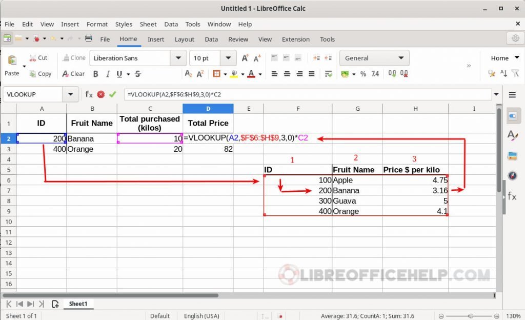
To calculate further, you can also fetch the price from the target table, put it in column D, and multiply the total quantity to calculate the price.

Then drag the cell handle down to fill up the rest of the cells with the formula.

Also, make sure to change the cell reference as global by adding “$” to prevent it from incrementing, which changes the search table. This is called an absolute reference. You can achieve it via pressing F4 while keeping the cursor in the target cell.

So, the final formula becomes this:

=VLOOKUP(A2,$F$6:$G$9,2,0)

=VLOOKUP(A2,$F$6:$H$9,3,0)*C2

Here’s the working flow and the final result.

HLOOKUP

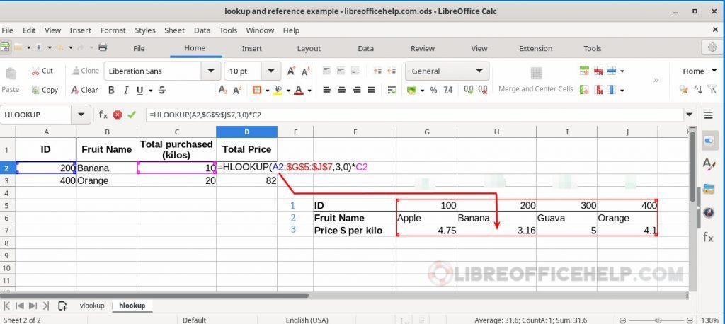
The next function is the horizontal lookup (or HLOOKUP). The HLOOKUP one is exactly opposite to VLOOKUP explained above.

So, this function searches left to right instead of searching top to bottom. That said, here’s the result of the exact same example above.

=HLOOKUP(A2,$G$5:$J$6,2,0)

=HLOOKUP(A2,$G$5:$J$7,3,0)*C2

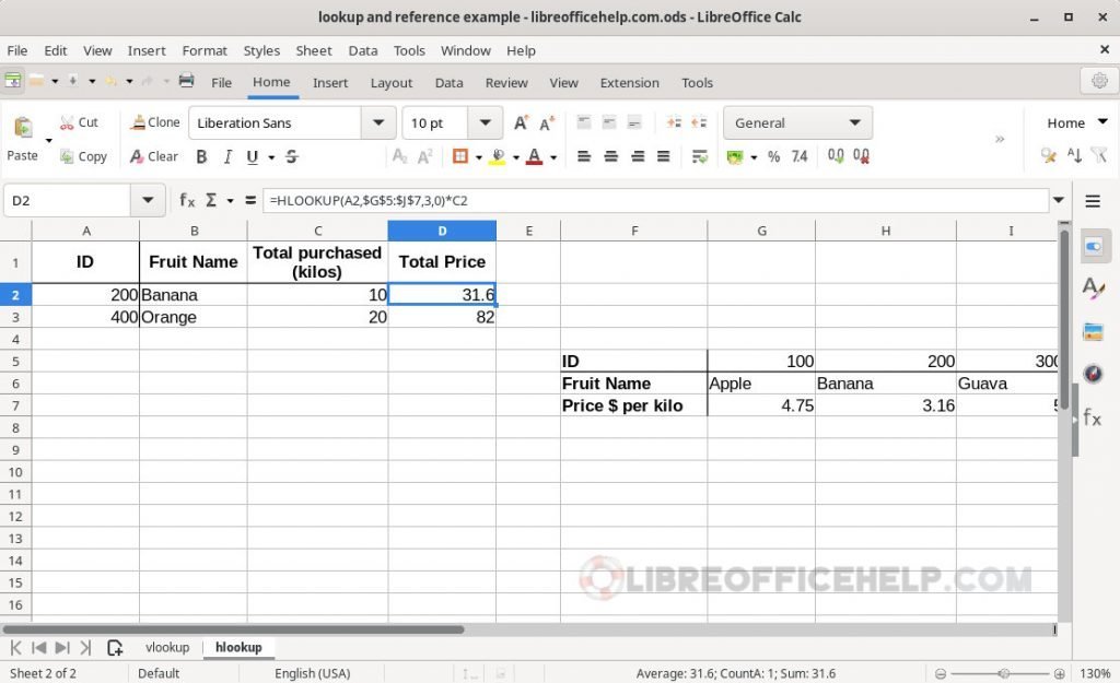
As you can see, the results are precisely the same.

INDEX and MATCH

The beauty of Calc is you can get the above same result using INDEX and MATCH functions. You do not need the lookup functions.

Here’s the syntax of both functions.

=INDEX(reference, row, column,[range])
reference: Table/range from where the data would be picked up
row: Row number of the above reference table
column: Column number of the reference table

=MATCH(search criteria, lookup array, type)
search criteria: the value to be searched
lookup array: single dimension array for search (e.g. one column)
type: 0=exact match 1=approximate match

So, to get the same result as above, you can use the two following formulas.

=INDEX($F$6:$G$9,MATCH(A2,$F$6:$F$9,0),2)

Explanation: Return the value from table F6 to G9. The row number is found by MATCH(), which is 2. And the column number is entered as 2 since we need to return the value from the G column.

=INDEX($F$6:$H$9,MATCH(A2,$F$6:$F$9,0),3)*C2

Explanation: Similarly, applying the same concept can return the price by mentioning the column number as 3.

Wrapping Up

This guide taught you the basics of various lookup reference functions in LibreOffice Calc. All the demonstrated functions above return the same result. It’s up to you which one you want to use for your use case.

Do let me know in the comment box below if it helps or if you may have any questions.