This tutorial explains the basics of SUMIF and SUMIFS functions in LibreOffice Calc.
Table of Contents
SUMIF
SUMIF Function returns the sum total of the values from a range/list of cells based on a condition. For example, if you have a list of numbers in Calc and want to sum only the values which are less than 20, then you can use the SUMIF function.
Here are some examples that will help you understand the workings of SUMIF.
SUMIF Examples
Using Numbers
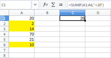
The below example sums the values from cells A1 to A6 if it is less than 20. The yellow highlighted values are the cells which are matching with the conditions.
=SUMIF(A1:A6,"<20”)
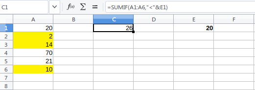
You can also keep the criteria value, i.e. 20 in a cell and use the cell reference in the SUMIF formula as below. It gives the same result as above.
=SUMIF(A1:A6,"<"&E1)
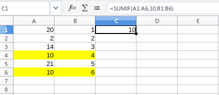
SUMIF can take three arguments where, based on the criteria, match in a range, you can sum another range. In the example below, it searches 10 in A1 to A6 and returns corresponding sums from range B1 to B6 if a match is found.
=SUMIF(A1:A6,10,B1:B6)
Similarly, you can put a value of 10 in any cell and use the cell reference in the above formula.
Using Texts
You can also search texts in a similar way and return the sum.
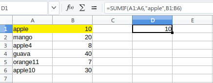
The following example searches “apple” in the range A1:A6 and returns the sum of matching entries from the corresponding sum range.
=SUMIF(A1:A6,"apple",B1:B6)
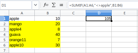
Using the condition below, you can sum the values that are NOT equal to a specific text/string. The NOT operator is <>. Please note that <> operator is inside the text with ".
=SUMIF(A1:A6,"<>apple",B1:B6)
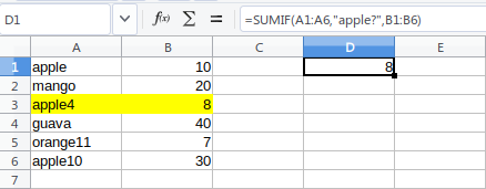
To search using a single wild card character, you can use ? in the condition. E.g. if you want to sum only strings matching with “apple4” and not “apple10” or “apple”, use the below example.
=SUMIF(A1:A6,"apple?",B1:B6)
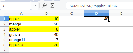
You can also use wild card * to search any number of characters in a range of cells and return the sum using SUMIF. The below example sums all matching cells where the apple word is found.
=SUMIF(A1:A6,"*apple*",B1:B6)
SUMIFS Example
You can use SUMIFS for multiple criteria ranges for summing up values. SUMIFS takes the first argument as the range to be summed and the next set of criteria as per the above examples.
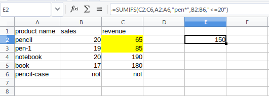
In the below example, it returns the sum of revenue when sales are less than or equal to 20, and the product name starts with pen.
=SUMIFS(C2:C6,A2:A6,"pen*",B2:B6,"<=20")
Note:
- SUMIFS conditions are evaluated as AND, and the sum is returned only when all conditions are satisfied.
- SUMIFS conditions ranges should be of the same length.
- You can specify at most 127 condition pairs in SUMIFS.
Summary
In conclusion, I guess this guide helped you to understand the working principles of SUMIF and SUMIFS. You can experiment with more conditions as per your need in LibreOffice Calc.
Drop a comment below if you have any questions or if this tutorial helped you.

I am not able to get sumif to work when comparing to cells with text/string contents. It works fine if I compare to “apple” but not if I compare to cell C5 which contains the word “apple”,. Am I overlooking something?
The formulas on this guide are not working for me (Libreoffice Version: 6.0.7.3 Ubuntu), I had to replace the commas with semicolons.
maybe because of your language. in my case( brazil), we also need to change it, because we use comma to separate decimals
It should work with both comma and semicolons.
It would be great if it functioned… ?
I cannot use dates to compare, although internally they are only integer values (the value is always 0 when I try to use dates). I cannot use wildcards on text comparations (the result is always 0 when I try to use text with wildcards)…
I’m using 6.2.6.2 LO version.
“sumifs” is so buggy…
I don’t think you can get too clever with SUMIF/S…
Today I wanted to compare the MONTH of the dates in column B to the headings of rows which contain dates… you cannot do the following:
=SUMIFS(C2:C100;MONTH(B2:B100);MONTH(D1);…;…)
The MONTH(B2:B100) piece is not a legal argument for the function.
I don’t find the SUMIF/S and COUNTIF/S buggy at all. Fussy/limited, yes, but not buggy.
Very new to using a spreadsheet and have very limited knowledge how to resolve this. Attempted to solve this with IF and IFS and SUMIF which seemed like it might be the best way. If you could point me in the correct direction it would be appreciated.
D3 is “yes” or “no” (this is a manual entry, effectively true or false)
If “yes” F3 = C3/B3
If “no” G3 = G3+C3
You can simply do it using IF function. No need SUMIF. SUMIF required when you need to sum based on conditions.
As per your comment:
Put this in cell F3
=IF(D3="yes",C3/B3)Put this in cell G3
=IF(D3="no",G3+C3)I think there’s an error on your last line. I assumed it is supposed to say
If “no” F3 = G3+C3
F3 needs the following formula, which presumes anything “non-YES” is a NO:
=IF(D3=”YES”;C3/B3;G3+C3)
Otherwise:
=IF(D3=”YES”;C3/B3;IF(D3=”NO”;G3+C3;””))
I am trying to get this to work. I have 38 sales entries
=SUMIFS(Cost, Date, “>”L6, Date,”<"N6, Client,=L4, Service,=$Data.A7)
Cost is the range to be summed
Date is the date of the transaction
L6 is the start date
N6 is the end date
Client is the range containing the client name
L4 is the client name I am trying to sum the transactions for
Service is the range containing various service types
$Data.A7 is where the various service types are stored
Hello,
I’m stuck with a SUMIFS with conditions on date with the date range coming from an imported file that might not be in proper date format, so I use DATEVALUE on the date range but then it stop working. If I create a new col with only the formula DATEVALUE on the date range and then use this new col as a range, it works again. If I manually format back all date in date col it works again as well.
So the question is: how to use DATEVALUE on the range criteria without getting an error?
Any help is welcome.
I’ve been using the SUM(SUMIFS()) function in an Excel spreadsheet for a year, and it works fine there. Transferring that spreadsheet to Calc 7.0.4.2.(x64), the function does not work as expected. After some experimentation using the formula =SUM(SUMIFS(E4:E11,D4:D11,{“complete”,”pending”})) from https://exceljet.net/formula/sumifs-with-multiple-criteria-and-or-logic, I found that it only returns the sum of cells meeting the first given condition (“complete”). There has to be something wrong in the Calc program, because the formula works fine in Excel. As this is my first time on this website, please let me know if this is not the right place to report the problem. Thanks.
multiple criteria for a single cell do not work as documented here – Error 504